


One area of research related to information retrieval that has received some attention is that of applications that employ statistical term co-occurrence. For the most part, term co-occurrence has been used as a query expansion technique. The general approach has been to expand a user's submitted query with ``synonyms'' which have been found to co-occur with the terms actually submitted. Overall, this technique has met with mixed results [Lesk1969,Sparck-Jones1971,Robertson et al.1981,Salton1986,Peat & Willett1991].
Another area, which has also received a good deal of attention, though only sporadically from the perspective of information retrieval, is that of lexical collocation. A lexical collocation, defined broadly, ``is an arbitrary and recurrent word combination'' [Benson1990]. In addition to being arbitrary and recurrent, lexical collocations are domain dependent and tend to form cohesive clusters [Smadja1993]. By cohesive clusters, we mean that the appearance of one (or more) part of the collocation tends to suggest the rest of the collocation, that the presence of one part offers ``evidence'' for the possible presence of the whole collocation.
In the case of lexical collocations, where such events are typically words, the higher the strength of the association between the occurrence of two (or more) words in some syntactic relation, the higher the probability that the collocation is important as evidence. In terms of purely statistical approaches, the ``syntactic relation'' can be relaxed to mean ``appear in linear succession in the same sentence''. In the case of co-occurrence query expansion, the terms are not as a rule constrained to be in any sort of syntactic or semantic relation (though this is clearly the intent), and hence, tend to produce only marginal results. Those experiments which do show good results are those which constrain the associations to a greater extent [Rada & Bicknell1989].
In the present discussion, we will be dealing with collocations not in the usual sense of lexical adjacency, but in a broader sense of document features which have a measurable association.
In the following two sections, we follow closely Dunning's presentation and
notation for non-parametric statistical techniques applied to word
collocations [Dunning1993]. At the heart of these techniques is the
observation that when events that co-occur with greater frequency than can be
accounted for by chance, they are likely to be highly associated. Given two
events A and B, if the probability P that they will appear together is
greater than the probability that they will appear independently, 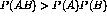 , then they are to some degree positively associated. If, on the
other hand, A and B are independent, then
, then they are to some degree positively associated. If, on the
other hand, A and B are independent, then 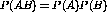 , these
probabilities are equal. The intent is not just to determine if two events
are associated, but to measure the strength of the association and thereby
highlight certain highly associated pairs of events.
, these
probabilities are equal. The intent is not just to determine if two events
are associated, but to measure the strength of the association and thereby
highlight certain highly associated pairs of events.
For our statistical analysis below, we construct a contingency table which contains the counts for each of the possible combinations of events A and B of the form:

where `` '' denotes the absence of some event. The possible
combinations are AB, where the events both occur;
'' denotes the absence of some event. The possible
combinations are AB, where the events both occur;  , where event A
occurs without B;
, where event A
occurs without B;  , where B occurs without A; and finally,
 where neither A nor B occurs.
For the training phase of this research, we take event A to be some lexical item (document subcomponent) identifiable in the document at hand (words or phrases taken variously from the titles, authors or abstracts), and event B to be a member of a list (set) of controlled vocabulary subject headings which has previously been assigned to that document by a human indexer. Such a formulation allows us to determine to what degree the lexical components of a particular document are highly associated with which members of the controlled vocabulary. However, for the deployment phase, we need to go further. First, when trying to predict which controlled vocabulary subject heading ought to be associated with a particular document, we need to reason not from a single lexical item (as might be the case with a single word title) but from several lexical clues. Lexical clues can be drawn from the words in a title or abstract or both. Second, we don't need to determine which event pairs are or are not correlated as much we need to rank the correlations. Fortunately, the statistical measure of correlation can be used quite naturally to deal with both of these concerns.
One of the problems in applying some standard statistical tests, such as the
 and z-score tests, to text is the assumption that the random
variables being sampled, the words of the text (or texts), conform to these
distributions. Such tests break down because of the large proportion of
``rare'' events, i.e. words that occur infrequently, in text. It has long
been recognized in information retrieval research that the frequency of words
in texts follows a Zipf curve:
and z-score tests, to text is the assumption that the random
variables being sampled, the words of the text (or texts), conform to these
distributions. Such tests break down because of the large proportion of
``rare'' events, i.e. words that occur infrequently, in text. It has long
been recognized in information retrieval research that the frequency of words
in texts follows a Zipf curve: 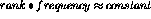 [Luhn1958,Salton1989]. This means that the so-called ``rare'' events in
text are very common. For example, Salton reports a sample of
[Luhn1958,Salton1989]. This means that the so-called ``rare'' events in
text are very common. For example, Salton reports a sample of  words of running text with 50,406 unique terms of which 22,543, nearly half,
occur only once [Salton1989]. The importance of such ``rare'' occurrences
are greatly overestimated by tests which assume a normal distribution.
words of running text with 50,406 unique terms of which 22,543, nearly half,
occur only once [Salton1989]. The importance of such ``rare'' occurrences
are greatly overestimated by tests which assume a normal distribution.
In order to avoid this problem, we cast the training part of our experiment as
a binomial event counting problem where each event A being counted is
compared to a particular event B. This allows us to measure the
independence of events A and B from each other by comparing the
distribution of event A given event B,  , to the distribution of
event A given the absence of B,
, to the distribution of
event A given the absence of B,  , where A is some clue
(lexical item) in the particular document at hand and B is a controlled
vocabulary subject heading which has previously been assigned to this document
by a human indexer. We take
, where A is some clue
(lexical item) in the particular document at hand and B is a controlled
vocabulary subject heading which has previously been assigned to this document
by a human indexer. We take  as the null hypothesis that A
and B are independent and compare their observed distributions to determine
the strength of association between them.
as the null hypothesis that A
and B are independent and compare their observed distributions to determine
the strength of association between them.
For this purpose we adopt the likelihood ratio for comparing these two
binomial processes as developed by Dunning as our test statistic
[Dunning1993]. The generalized likelihood function is written as
 where
where  represents the model parameters (hypothesis) and
k the observations being tested. The likelihood ratio is the maximum value
of the likelihood function for the particular hypothesis being tested over the
maximum value of the function over the entire parameter space
represents the model parameters (hypothesis) and
k the observations being tested. The likelihood ratio is the maximum value
of the likelihood function for the particular hypothesis being tested over the
maximum value of the function over the entire parameter space

where  is the hypothesis being tested and
  is the
entire parameter space. In the current case, the likelihood function for a
binomial process is given as
is the
entire parameter space. In the current case, the likelihood function for a
binomial process is given as

where p is model parameter (expected probability of a particular outcome), k, the number of positive observations and n the total number of observations. This likelihood ratio for such a function is the maximum value of this function for the hypothesis being tested over the maximum value of the function over the entire parameter space. For two binomial processes, the function becomes

By using this function to test the null hypothesis that the parameters  and
and  are equal, we can use it in the likelihood ratio. The maximum
value of this function over the entire parameter space (i.e. the two binomial
processes) is the observed ratio of positive observations to total
observations for each process
are equal, we can use it in the likelihood ratio. The maximum
value of this function over the entire parameter space (i.e. the two binomial
processes) is the observed ratio of positive observations to total
observations for each process  and
and  .
The maximum value for the particular hypothesis being tested, that
.
The maximum value for the particular hypothesis being tested, that  , is given as
  . That is,

which, after inserting the binomial functions, can be reduced to

The logarithm of this ratio gives

where

and as previously noted

At this point, the only unknown values,  and
and
 are the frequency observations taken directly from the contingency
tables.
are the frequency observations taken directly from the contingency
tables.  and
and  , correspond to the observed distribution of A
given B:
, correspond to the observed distribution of A
given B:  , the number of positive observations, and
  , the total observations.
  and
and  take their values
from the distribution of A given that B is not present:
take their values
from the distribution of A given that B is not present:  and
and 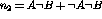 . For any given contingency
table, we can now easily calculate the
. For any given contingency
table, we can now easily calculate the  statistic. We
interpret this statistic as a ``weight'' of association between two events and
use it as a predictor of relevance between them, where the two events are a
lexical clue (A) and a controlled vocabulary subject heading (B).
statistic. We
interpret this statistic as a ``weight'' of association between two events and
use it as a predictor of relevance between them, where the two events are a
lexical clue (A) and a controlled vocabulary subject heading (B).
We also include a representative example using the  test as a
comparison to demonstrate the effectiveness of this method in
Section 5.1.
test as a
comparison to demonstrate the effectiveness of this method in
Section 5.1.